New Atmospheric Data Model for Flight Trajectory Optimization

Atmospheric Conditions: A Complexity Increasing Factor in Flight Trajectory Optimization

This article presents a research conducted at the Laboratory of Research in Active Control, Avionics, and AeroServoElasticity (LARCASE) on a new atmospheric data model for use in flight trajectory optimization applications, and the resulting paper published in a peer-reviewed journal ([1]). This investigation was part of the research conducted under the auspices of the Green Aviation Research and Development Network (GARDN) in the fields of aircraft flight performance identification and modelling ([2-4]), and flight trajectory optimization ([5-11]).

Atmospheric conditions (air temperature and wind) are an important factor in flight planning as they have a direct impact on engine performance (fuel burn rate, maximum thrust, etc.) and aircraft speed, both relative to the air mass (true airspeed) and the ground (ground speed). Engine performance and aircraft speed determine flight time, fuel burn and overall costs for the flight. Environmental concerns and economic factors, accentuated by the impact of COVID-19 on the aviation industry ([12, 13]), amplify the industry’s demand for better flight planning and flight trajectory optimization methods and techniques. One method to improve the flight trajectory optimization results is to devise better aircraft and atmospheric data models, i.e. more accurate and/or less computationally intensive, which would lead to more accurate estimations of flight performance parameters for a flight profile and/or more candidate flight plan evaluations during the optimization process. The work presented in the paper and highlighted here proposes an atmospheric data model, designed for constant altitude cruise optimization, which yields atmospheric parameters in selected points with the same precision and, on average, six times faster that when computed based on atmospheric data issued by meteorological agencies.

Available Forecast Data

The space-time variation of atmospheric parameters is very complex, even chaotic, and cannot be globally expressed by a unique set of equations. The method employed by the meteorological agencies to describe/approximate atmospheric parameters and their variation is based on piecewise functions. The forecast data is issued in a gridded format (GRIB2 [14, 15]), where the atmospheric parameter values are defined in the nodes of a four-dimensional grid: latitude, longitude, pressure altitude, and time. An atmospheric parameter in a point other than a grid node is computed by interpolation.

Meteorological agencies might issue various forecast data types, which differ as a function of the area covered by the forecast (global [16, 17] or regional [18, 19]), map projection (latitude-longitude or polar stereographic) and grid resolution, and update rate (how often the forecasts are issued). An illustration of air temperature and wind forecast data is the global forecast issued by Environment Canada on June 14, 2016, at 12:00 Universal Time Coordinate (UTC), on a longitude-latitude map with a 0.6° × 0.6° grid resolution, presented in Figure 1 and Figure 2. These figures show the forecast the data cropped to seven time instances, four pressure altitudes, and a region delimited by latitudes [15 °N, 75 °N] and longitudes [130.2 °W, 30 °E] domains. Figure 1 shows the air temperature (T) in terms of ISADEV: air temperature deviation relative to standard atmosphere ([20, 21]) air temperature at that particular altitude. Figure 2 shows the wind patterns (speeds and directions). The forecasted wind data could be specified as vectors (wind speed W and heading αW relative to the geographic North) or wind components along the geographic North (WU) and East (WV) axes.

Figure 1 Example of ISADEV variation with altitude and geographic location for a set of pressure altitudes, based on the air temperature forecast issued by Environment Canada for June 14, 2016

Figure 2 Example of wind vector (speed and direction) variation with altitude and geographic location for a set of pressure altitudes, based on wind
forecast issued by Environment Canada for June 14, 2016

Computational Complexity in Flight Trajectory Optimization

A flight trajectory optimization is performed by iteratively generating candidate flight trajectories and evaluating their performance parameters. The flight performance for a flight trajectory is evaluated by decomposing it in a relatively large number of small sub-segments (integration steps) and, then, the flight performance parameters are successively evaluated for each sub-segment. Each sub-segment performance calculation requires an evaluation of the atmospheric parameters (air temperature and wind).

In flight trajectory performance calculations and flight trajectory optimization applications, the atmospheric data in a point of interest (a particular aircraft location: latitude, longitude, altitude, and time) are calculated using four-dimensional linear interpolations ([22, 23]) — a trade-off between accuracy and computational complexity/time ([23]). Even so, this operation is computationally expensive/time consuming (equivalent to 15 linear interpolations). A wind evaluation in a point of interest requires two four-dimensional interpolations: one for each component (WU and WV).

By reducing the atmospheric parameter computational complexity while maintaining result accuracy, it is possible to perform more flight profile evaluations in a given time or to obtain the optimal profile more rapidly (for a fixed number of profile evaluations). This could yield better and/or faster optimization results.

Proposed Atmospheric Data Model

The development of the proposed atmospheric data model (ADM) started from the observation that if an independent parameter of an n-dimensional linear interpolation is fixed, the expression of the parameter variation can be reduced to one equivalent of a (n-1) dimensional interpolation.

The candidate flight trajectories for a constant altitude cruise section could be constructed by selecting adjacent nodes from a routing grid (illustrated in Figure 3 and Figure 4), where the routing grid is constructed so that the distance between two such nodes (the segment length) is smaller or equal to the distance integration step used in the flight trajectory performance calculation. In this case, each node of the routing grid is situated at a fixed latitude, longitude, and pressure altitude. It is therefore possible to express the atmospheric parameters’ variation in a grid node only as a piecewise function of time.

Figure 3 Example of a flight trajectory constructed based on a routing grid, and the wind structure at a selected altitude

Figure 4 Example of a flight trajectory constructed based on a routing grid, and the ISADEV structure at a selected altitude

For each routing grid node and time domain, the coefficients in the expression for a parameters’ linear variation could be computed once and stored in memory. From a mathematical point of view, the four-dimensional interpolation and the proposed method are equivalent; the model’s coefficients are in fact intermediary results, obtained at the end of the first three steps of the four-dimensional interpolation. Therefore, it is expected that the proposed method yields results identical to those obtained from a four-dimensional interpolation.

Evaluation of the Atmospheric Data Model

The proposed data model was evaluated using four routing grids, which differ in terms of maximum distance between adjacent grid nodes (grid step sizes along and across the orthodromic route), maximum number of lateral steps, and the maximum deviation relative to the orthodromic route. Consequently, the number of routing grid points was different for each grid. The grid was constructed based on the geographic locations of the beginning and the end of the cruise phase of a real flight (Air Transat 601, flown on June 14, 2016 [24]) retrieved from the FlightAware website. The time span for the ADM was taken as the GRIB time domain that covers the estimated range of aircraft flight time on the cruise section.

These test scenarios allowed to evaluate:

• The memory space required for storing the ADM, relative to GRIB data, for the same geographic area and forecast time domain;
• The time required to generate the ADM for different grid sizes;
• The computation time reduction, when an accelerated flight trajectory performance calculation is done using the ADM versus GRIB data.

The accuracy of the ADM and the computation time reduction were evaluated by comparing atmospheric parameter values and computation times, when generated using the ADM, with their values obtained when using the GRIB data. The evaluations were performed for 137,520 test cases, a set of 133 time instances for each node of a grid. Results showed that the atmospheric parameter values are identical (differences of the order of 10-14). On average the atmospheric parameters were computed six times faster than based on the GRIB data. Figure 5 shows the GRIB versus ADM computation time ratio distribution:

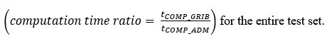
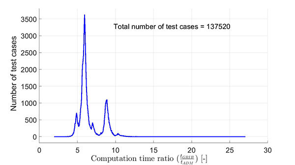
Figure 5 Computation time ratio GRIB versus ADM

The cost of atmospheric parameter computation time improvement is an increase in the memory footprint for the model data. However, for lower-resolution grids (larger distances between the nodes) the memory footprint was smaller than for GRIB data.

The overall flight trajectory computation time reduction using the ADM atmospheric data model, relative to using GRIB data, was evaluated by performing two sets of accelerated flight trajectory performance calculations, under the same conditions (flight trajectory, altitude, etc.): one using the ADM and the other using the GRIB data. Results showed a flight trajectory performance calculation time improvement of up to 22%.

Conclusion

The atmospheric data model, presented in the paper referenced in this article, can provide atmospheric data in a set of airspace locations (longitude ‒ latitude points), at a selected altitude, for time instants within a time domain for which the model was created. The atmospheric parameters computed using the proposed model have the same accuracy as when computed from the GRIB forecast data issued by meteorological agencies, but is six times faster on average. A shorter evaluation time for a candidate flight plan means that the optimization process could be faster or more candidate flight profiles could be evaluated per allotted time. Better optimization results mean that the flight trajectory solutions yield lower fuel burn (therefore, lower polluting emissions) and/or costs, with a positive impact on the environment and economic performance of the aircraft operator.

Additional Information

For additional information on this research and the research conducted at the Laboratory of Research in Active Control, Avionics, and Aeroservoelasticity (LARCASE) please visit the LARCASE website and read the published article on this subject ([1]).